In the second installment of the SIGGRAPH Series, I have shown you how the MANN model works. Now it is time to download and understand the repo provided by the authors.

Controlling characters in real time demands a system to blend their movements according to the user’s input. Historically this was done with a state machine and algorithms that help optimize the transition pose. But this is a problem that could be simplified using neural networks.

In 2017 Holden et al. achieved good results could using if different networks were used to learn separate parts of the movement. Now Zhang, Sebastian, et al. generalize that approach to quadrupeds, a harder problem to solve. I have created a short video outlining the proposed model; you can watch the video clicking here. This article is meant as support material to that video, so I encourage you to watch it first.

The authors have generously made their data and code available. This article is meant as a guide to their repository, so you can understand it and use it with your own datasets. Here is what you will learn:

1. Set the project up with the default [Neural Net] weights
2. Training the neural network with the original data
3. Highlights in the neural network implementation
4. Pre-process new data to train the network
5. Highlights in the pre-processing implementation
6. Training the neural network with your own data

Helpful resources

Set the project up with the default weights

As you have seen in the video, the authors provide a compiled version of the demo for Windows, Linux, and macOS. But you can download the source Unity project from the repo. If you do, so I recommend you use Unity version 2018 1.2.f, so you don’t get any errors or warnings.

When you load the project, you’ll notice the character won’t move because the trained Neural Network weights don’t come bundled with the repo. You can download them using the link I provide in the resources for this article, or in the link found in the repo itself.

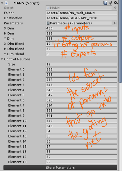
Note, that there are 58 different files. Out of those 54 hold the weights and biases for each layer in the network: 8 specialist networks * (2 hidden layers + 1 output layer each) + (2 hidden layers and 1 output layer in the gating network) * 2 [for weights and biases]. The other 4 files hold the mean and standard deviations for the normalization of inputs and outputs. The files follow this naming convention:

• Layers of the Motion Prediction network
  • start with ‘cp?_’ where ? is the layer number
  • end with ‘a?’ or ‘b?’ where a is for the weights, b for the biases and ? is the expert number
• Gating network
  • start with ‘wc?’ where ? is the layer number
  • end with w or b, where w is for the weights, and b for the biases
• Normalization
  • X for inputs, Y for outputs, mean for feature wise means, and std for feature wise standard deviations

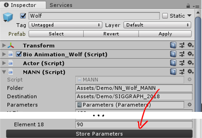
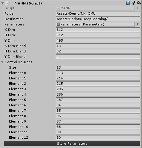
Once you have downloaded and extracted the files to your disk,  select the Wolf prefab in the Unity demo-scene and look for the ‘Folder’ parameter in the MANN (Script) component. Change the folder to the path where you have extracted the files and press ‘Store Parameters’. Now your Unity project should be on par with the compiled version.

Training the Neural Network

If you want to fiddle with the network’s configuration, you can train it yourself using the pre-processed dataset provided by the authors. The link for the dataset can be found in the repo itself as well as in the resources for this article. The Input.txt and Output.txt files should be downloaded and stored in the AI4ANIMATION/TensorFlow/2018/data folder.

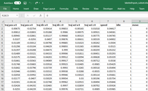
You’ll notice that this data is a bit hard to grasp as there are no labels. For didactic purposes, I’m providing an Excel file with a labeled subset of that data. Notice that every trajectory point in the inputs is 13 dimensions long (2d position, 2d direction, 2d velocity, 1d speed, 6d style [one hot encoded]) and every bone in the body is 12 dimensions long (3d position, 6d orientation, 3d velocity). In the outputs, trajectory points are 6d long (2d position, 2d direction, 2d velocity), bones in the body are 12 dimensions long, and there is a final 3d vector for the root displacement.

The authors trained the Neural Network in TensorFlow. TensorFlow is Google’s deep learning library which has a Python interface. TensorFlow is the most popular deep learning library out there, and I have previously discussed why I have not used TensorFlow in other tutorials: Python3 and Maya don’t go well together. But we are using TensorFlow under the hood every time we run Keras code in Google Colaboratory.

To run the training code in this repo, you’ll need to install Python 3 (link here) if you haven’t already. After installing Python 3, add it to your PATH environment variable like you have done with Mayapy.exe in this previous tutorial. If you have other Python installations in your PATH a hacky way to avoid conflicts is to rename your python.exe to python3.exe. Do it at your own risk.

Then you’ll need to install Numpy and TensorFlow in your Python3 interpreter, run this code:

python -m pip install numpy
python -m pip install tensorflow

From my tests, I can safely say that training this network with the original dataset using the CPU is not viable. You can if you want to see TensorFlow working, but don’t expect to get more than one epoch per hour even with a fast CPU. So, I highly encourage you to install TensorFlow’s GPU implementation. First check that you have a Nvidia 600+ GPU, anything older than that is not compatible with CUDA 9.0, the CUDA version used by TensorFlow. If you meet that criteria install CUDA 9.0 toolkit (link here) and only then proceed to install TensorFlow GPU, like this:

python -m pip install –upgrade tensorflow-gpu

Finally, in a command prompt change directory to the AI4ANIMATION/TensorFlow/2018 folder and run main.py.

python main.py

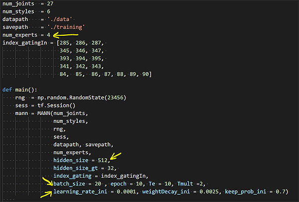
You might get TensorFlow to crash at you if your GPU’s memory is not large enough to fit a batch into memory. A batch is a subset of the dataset that is used to train the network. Ideally, we would fit all the data into memory, but that is not always possible. The default batch_size (main.py, line 19) for this code is 32, so that means the ~250,000 samples of 843 scalars (inputs+outputs) are divided into batches of ~7,800 samples and fed to memory. That was too large for my GTX670, I’ve reduced the batch_size to 20, and it worked. You’ll have to see what works for you; maybe you can even increase it.

You can also play with the number of epochs, the number of hidden layers, the number of experts and the learning rate to explore other concepts that we have discussed in this and previous articles. This parameters can be all configured in the main.py file.

If you want to load the weights of the network you have trained copy the files generated by TensorFlow in the AI4ANIMATION/TensorFlow/2018/training/nn, and AI4ANIMATION/TensorFlow/2018/training/normalization folders, into one single folder and load that in the Wolf demo scene, like I’ve shown before. Note that if you have changed parameters such as the number of experts or the number of neurons you’ll have to replace those in Unity as well before importing the weights. Use the following image as a guide:

If you want to pre-process your own data skip to the next section. If you want to learn more about the code that trains the network, stay with me.

Highlights in the Neural Network implementation

Before dissecting the code that was used to train the model, a warning. This model was built on TensorFlow’s default API, which is very flexible but demands a lot more lines of code than Keras (the framework I’ve been using in previous tutorials). In TensorFlow you must implement some operations that are implicit in Keras.

Now that you know that let’s see how the authors use TensorFlow to build the model. First, they initiate a gating network.  From the gating network, we expect to get the BC parameter, that is, the Blending Coefficients for the experts in the Motion Prediction network. From MANN.py :

class MANN(object):
[…]
       def build_model(self):
[…]
        """BUILD gatingNN"""
        #input of gatingNN
        self.input_size_gt = len(self.index_gating)
        self.gating_input = tf.transpose(GT.getInput(self.nn_X, self.index_gating))
        self.gatingNN = Gating(self.rng, self.gating_input, self.input_size_gt, self.num_experts, self.hidden_size_gt, self.nn_keep_prob)
        #bleding coefficients
        self.BC = self.gatingNN.BC

The Gating network is defined in Gating.py. It is a 2 hidden layer neural network with a soft-max for output. The soft-max layer makes the sum of all activations equal to 1 while making the winner stand out. This is a great behavior for what we expect from the Blending Coefficients.

The BC parameter of the Gating network is just an alias for its feed-forward (FF) operation, that is, the model’s prediction. As I have said before, in TensorFlow, you need to write more code… You actually have to implement the net’s feed forward by yourself. In the code below H0 is the input layer, H1 the first hidden layer, H2 the second hidden layer and H3 the network’s output. At every layer (after the input) the layer’s inputs and weights are multiplied and the neuron biases are added. Then the activation function ELU is applied, I have not mentioned ELU before, but it is an activation function much like TANH and SIGMOID. Finally, the authors use a dropout. Dropout is a technique to increase the network’s ability for generalization by throwing away a random samples; it sounds counter-intuitive, but it works. We’ll probably discuss dropout in a future article but you can Google it.

class Gating(object):
[…]
        """"output blending coefficients"""
        self.BC = self.fp()
[…]
    """forward propogation"""
    def fp(self):
        H0 = tf.nn.dropout(self.input, keep_prob=self.keep_prob) #input*batch
        
        H1 = tf.matmul(self.w0, H0) + self.b0 #hidden*input mul input*batch
        H1 = tf.nn.elu(H1)
        H1 = tf.nn.dropout(H1, keep_prob=self.keep_prob)
        
        H2 = tf.matmul(self.w1, H1) + self.b1
        H2 = tf.nn.elu(H2)
        H2 = tf.nn.dropout(H2, keep_prob=self.keep_prob)
        
        H3 = tf.matmul(self.w2, H2) + self.b2 #out*hidden mul hidden*batch
        H3 = tf.nn.softmax(H3,dim = 0) #out*batch
        return H3

Back to the model definition in MANN.py the hidden layers and output layers of the network are initialized using a custom set of weights built by the authors: ExpertWeights. ExpertWeights is a class that creates N sets of weights and biases for the network. From MANN.py, line 83:

        #initialize experts
        self.layer0 = ExpertWeights(self.rng, (self.num_experts, self.hidden_size, self.input_size), 'layer0') # alpha: 4/8*hid*in, beta: 4/8*hid*1
        self.layer1 = ExpertWeights(self.rng, (self.num_experts, self.hidden_size, self.hidden_size), 'layer1') # alpha: 4/8*hid*hid,beta: 4/8*hid*1
        self.layer2 = ExpertWeights(self.rng, (self.num_experts, self.output_size, self.hidden_size), 'layer2') # alpha: 4/8*out*hid,beta: 4/8*out*1

To get the blended weights of each layer, we get_NNWeight from an ExpertWeight layer using the BC parameter (output of the gating network). And we do the same for the biases. From MANN.py, line 93:

        w0 = self.layer0.get_NNweight(self.BC, self.batch_size)
        w1 = self.layer1.get_NNweight(self.BC, self.batch_size)
        w2 = self.layer2.get_NNweight(self.BC, self.batch_size)
        
        b0 = self.layer0.get_NNbias(self.BC, self.batch_size)
        b1 = self.layer1.get_NNbias(self.BC, self.batch_size)
        b2 = self.layer2.get_NNbias(self.BC, self.batch_size)

Finally, the authors define the feed-forward operation for the network, which is much the same operation they’ve implemented for the gating network, except there is no activation function in the end, which is ok since this is a regression network. MANN.py, line 102:

        #build main NN
        H0 = tf.expand_dims(self.nn_X, -1) #?*in -> ?*in*1
        H0 = tf.nn.dropout(H0, keep_prob=self.nn_keep_prob)
      
        H1 = tf.matmul(w0, H0) + b0 #?*out*in mul ?*in*1 + ?*out*1 = ?*out*1
        H1 = tf.nn.elu(H1)
        H1 = tf.nn.dropout(H1, keep_prob=self.nn_keep_prob)
        
        H2 = tf.matmul(w1, H1) + b1
        H2 = tf.nn.elu(H2)
        H2 = tf.nn.dropout(H2, keep_prob=self.nn_keep_prob)
        
        H3 = tf.matmul(w2, H2) + b2
        self.H3 = tf.squeeze(H3, -1) #?*out*1 ->?*out

Neural Network runtime implementation

In our previous tutorials, we have used the same model implementation for training and prediction. That is possible because we can call the predictions using Python within Maya. But the authors used Unity as a platform, where Python is not available. In this case, they could either deploy their trained method as a C++ library or recreate the Neural Networks in C# (Unity’s scripting language) and load the trained weights. The authors chose the latter. They have wrapped a C++ linear algebra library (Eigen) so as to not re-write everything from scratch, and I guess, for performance reasons.

You can find building blocks for building the final model in the Scripts/DeepLearning folder. Tensor.cs and Parameters.cs scripts describe the basic data types for storing and manipulating the networks inputs, weights, and biases. While NeuralNetowrk.cs is a class built to define Neural Nets with layers, activations, and so on. All models in the Scripts/DeepLearning/Models folder are instances of the NeuralNetwork type.

The MANN Model (MANN.cs) has functions to store (StoreParametersDerived) and load (LoadParametersDerived) the network’s parameters. These are the methods we have called when loading the original network weights provided by the authors. After defining these methods, the authors declare the feed-forward operation in the Predict() method. From MANN.cs:

public class MANN : NeuralNetwork {
[…]

        public override void Predict() {
            //Normalise Input
            Normalise(X, Xmean, Xstd, Y);

            //Process Gating Network
            for(int i=0; i<ControlNeurons.Length; i++) {
                BX.SetValue(i, 0, Y.GetValue(ControlNeurons[i], 0));
            }
            ELU(Layer(BX, BW0, Bb0, BY));
            ELU(Layer(BY, BW1, Bb1, BY));
            SoftMax(Layer(BY, BW2, Bb2, BY));

            //Generate Network Weights
            W0.SetZero(); b0.SetZero();
            W1.SetZero(); b1.SetZero();
            W2.SetZero(); b2.SetZero();
            for(int i=0; i<YDimBlend; i++) {
                float weight = BY.GetValue(i, 0);
                Blend(W0, CW[6*i + 0], weight);
                Blend(b0, CW[6*i + 1], weight);
                Blend(W1, CW[6*i + 2], weight);
                Blend(b1, CW[6*i + 3], weight);
                Blend(W2, CW[6*i + 4], weight);
                Blend(b2, CW[6*i + 5], weight);
            }

            //Process Motion-Prediction Network
            ELU(Layer(Y, W0, b0, Y));
            ELU(Layer(Y, W1, b1, Y));
            Layer(Y, W2, b2, Y);

            //Renormalise Output
            Renormalise(Y, Ymean, Ystd, Y);
        }
[…]
}

As you can see these are the same operations defined in TensorFlow, with a different syntax. Note that first they feed-forward the gating layers, then they reset the motion predicting layers with the blended weights. Finally, they feed-forward the remaining layers.

Pre-process new data to train the network

You might want to go further with this repo and pre-process the training data yourself. I see two reasons for doing this: (1) you want to experiment fiddling with the input and output parameters for the network, and (2) you want to use MANN for your own dataset and applications. So, I’ll talk about these two possibilities, and will use the CMU dataset as an example of the latter.

If you want to stick to the authors’ dataset that’s ok, you can find the link for it in the resources. If you’re going to use clips from the CMU dataset I recommend you download subject 127, for it has the most compatible movements for this application (link the in the resources as well).

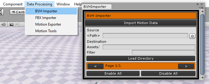
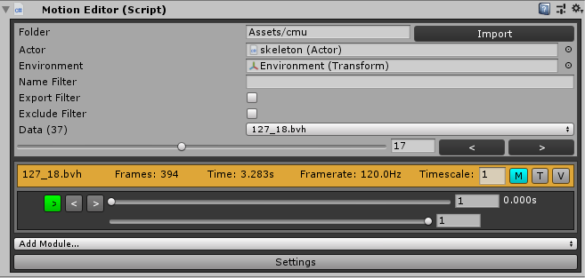
The first thing to notice is that the authors provide a BVH importer with this repo, which is excellent because many research MoCap datasets are available in that format. The BVH Importer and the Motion Exporter can be found under the Data Processing menu. After choosing the source and destination folders, select the clips you want to import and press ‘Import Motion Data’, the clips will be stored as assets in your Unity project.

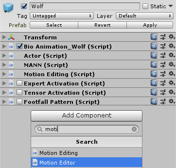
To load the animations, you’ll have to add the Motion Editor script as a component to your character. If you are using the author’s dataset, I suggest you start with the demo-scene provided in the repo. I recommend that because some adjustments need to be done to the character (like choosing which bones should be animated) that have already been done in that scene.

If you are proceeding with the CMU example, you can generate a skeleton from the BVH in MotionBuilder or use the one I provide you with the resources for this article. There is one gotcha you should be aware of when importing that FBX to Unity. Unity will rearrange the objects into alphabetic order like so:

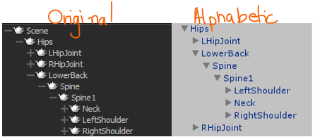
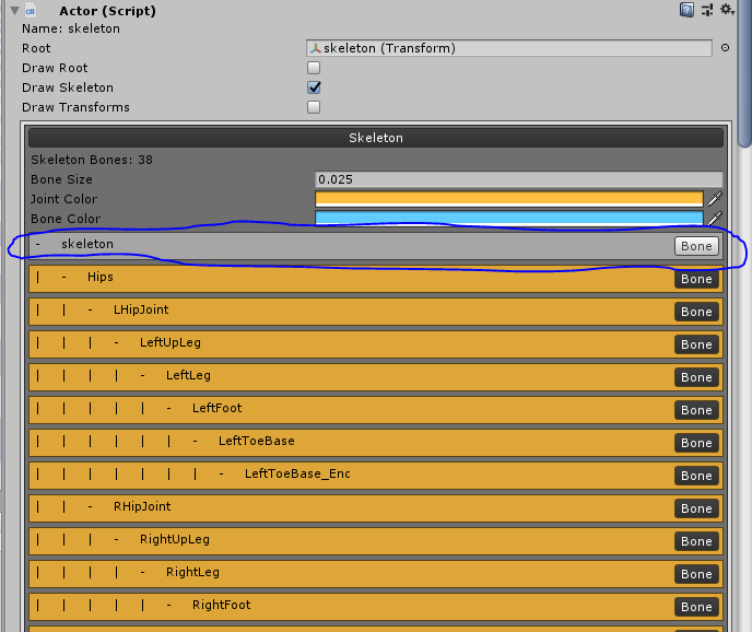
Since the Motion Editor script applies the motions by bone index and not by bone name, this will cause problems. So, rearrange the elements to the original order, as seen the image above. Also, disable the root bone named ‘Skeleton’ in the Actor component, as shown in the image below:

The motion editor is a modular tool for processing and annotating the data. Under settings, you can determine if that clip should be exported or not, amongst other things like the export frame range.

Under Add Module you can add annotation modules like the Style annotation used in the MANN paper or the foot contact annotation used in the PFNN paper. The Style module looks like this:

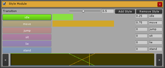
As you can see in the image above, you can add as many styles as you want, annotate the animation, create transitions and so on. It is very powerful, yet simple to use. In your first attempt to do this I encourage you to follow this template with 6 styles, in this exact order: idle, move, jump, sit, lie, stand. This is so you can use the character controller script provided by the authors.

Annotate as many clips as you want to use to train your network, but keep in mind it cannot learn things you don’t show it. So, for example, if you want it to learn how to transition from one style to another, move left, right, and so on, these actions need to be in your data. One more thing, having too many examples of one motion and too few of another can bias the training.

Before exporting the data, one more thing. As this is repo is continuously updated by the authors the MotionExporter.cs script does not produce the exact inputs and outputs used in the demo-scene any longer. Some things were removed (the speed for every trajectory point) and others added (the style for every output point). I recommend that, for this example, you substitute the MotionExporter.cs file with the one provided in the resources for this article.

When you are good to go, use the Motion Exporter provided in the Data Processing menu. If you want to train the network using this new dataset now, skip to the next section. If you want to know what the MotionExporter is doing under the hood, stay with me.

Highlights in the pre-processing implementation

The motion and the annotations (in this case, the motion style) are exported to CSV format via the MotionExporter.cs script. The script will loop through all frames in all files creating a State for the current frame and for the subsequent frame. From MotionExporter.cs, line 364:

for(int state=0; state<states.Count-1; state++) {
    Writing = (float)(state) / (float)(states.Count-2);
    State current = states[state];
    State next = states[state+1];
    editor.LoadFrame(current);

A State is a collection of information about an instant of time that is used to build the inputs and outputs to train the network. This information’s are Root xfo, Root Motion, Joint xfos, Joint velocities and the trajectory. The State also has a mirrored parameter for the mirroring the authors have used for data augmentation purposes. From the State.cs script:

public class State {
    public int Index;
    public float Timestamp;
    public bool Mirrored;
    public Matrix4x4 Root;
    public Vector3 RootMotion;
    public Matrix4x4[] BoneTransformations;
    public Vector3[] BoneVelocities;
    public Trajectory Trajectory;
[…]
   public State(Frame frame, bool mirrored) {
        Index = frame.Index;
        Timestamp = frame.Timestamp;
        Mirrored = mirrored;
        Root = frame.GetRootTransformation(mirrored);
        RootMotion = frame.GetRootMotion(mirrored);
        BoneTransformations = frame.GetBoneTransformations(mirrored);
        BoneVelocities = frame.GetBoneVelocities(mirrored);
        Trajectory = frame.GetTrajectory(mirrored);
   }
}

As you can see all the data is generated by a Frame object and stored in the State. Getting the xfos and deltas (root motion and bone velocities) is straightforward, so let’s study how Frame is generating the trajectory. From Frame.cs, line 185:

    public Trajectory GetTrajectory(bool mirrored) {
        StyleModule styleModule = Data.GetModule(Module.TYPE.Style) == null ? null : (StyleModule)Data.GetModule(Module.TYPE.Style);
        PhaseModule phaseModule = Data.GetModule(Module.TYPE.Phase) == null ? null : (PhaseModule)Data.GetModule(Module.TYPE.Phase);

        Trajectory trajectory = new Trajectory(12, styleModule == null ? 0 : styleModule.Functions.Length);

        //Current
        trajectory.Points[6].SetTransformation(GetRootTransformation(mirrored));
        trajectory.Points[6].SetVelocity(GetRootVelocity(mirrored));
        trajectory.Points[6].SetSpeed(GetSpeed(mirrored));
        trajectory.Points[6].Styles = styleModule == null ? new float[0] : styleModule.GetStyle(this);
        trajectory.Points[6].Phase = phaseModule == null ? 0f : phaseModule.GetPhase(this, mirrored);

Note that the current frame is stored as the 6^th (zero-indexed) point of the 12 points in the trajectory. So, there are 6 points before it, and 5 afterwards. These points are timestamped to cover one second in to the past and another second into the future (look for timestamp – delta and timestamp + delta). Note that the letter f (as in -1f + float(i)/6f) does not mean frames, but float. Also, note that one will have problems for both past and future if the current frame is not within one second of the beginning or the end of the animation. That is why the authors chose to first test if they are not sampling outside of the frame range, if that is the case they try to resample the points within the proper limits. From Frame.cs, line 198:

	//Past
	for(int i=0; i<6; i++) {
		float delta = -1f + (float)i/6f;
		if(Timestamp + delta < 0f) {
			float pivot = - Timestamp - delta;
			float clamped = Mathf.Clamp(pivot, 0f, Data.GetTotalTime());
			float ratio = pivot == clamped ? 1f : Mathf.Abs(pivot / clamped);
			Frame reference = Data.GetFrame(clamped);
			trajectory.Points[i].SetPosition(Data.GetFirstFrame().GetRootPosition(mirrored) - ratio * (reference.GetRootPosition(mirrored) - Data.GetFirstFrame().GetRootPosition(mirrored)));
			trajectory.Points[i].SetRotation(reference.GetRootRotation(mirrored));
			trajectory.Points[i].SetVelocity(reference.GetRootVelocity(mirrored));
			trajectory.Points[i].SetSpeed(reference.GetSpeed(mirrored));
			trajectory.Points[i].Styles = styleModule == null ? new float[0] : styleModule.GetStyle(reference);
			trajectory.Points[i].Phase = phaseModule == null ? 0f : 1f - phaseModule.GetPhase(reference, mirrored);
		} else {
			Frame previous = Data.GetFrame(Mathf.Clamp(Timestamp + delta, 0f, Data.GetTotalTime()));
			trajectory.Points[i].SetTransformation(previous.GetRootTransformation(mirrored));
			trajectory.Points[i].SetVelocity(previous.GetRootVelocity(mirrored));
			trajectory.Points[i].SetSpeed(previous.GetSpeed(mirrored));
			trajectory.Points[i].Styles = styleModule == null ? new float[0] : styleModule.GetStyle(previous);
			trajectory.Points[i].Phase = phaseModule == null ? 0f : phaseModule.GetPhase(previous, mirrored);
		}
	}

        //Future
        for(int i=1; i<=5; i++) {
            float delta = (float)i/5f;
            if(Timestamp + delta > Data.GetTotalTime()) {
                float pivot = 2f*Data.GetTotalTime() - Timestamp - delta;
                float clamped = Mathf.Clamp(pivot, 0f, Data.GetTotalTime());
                float ratio = pivot == clamped ?1f : Mathf.Abs((Data.GetTotalTime() - pivot) / (Data.GetTotalTime() - clamped));
                Frame reference = Data.GetFrame(clamped);
                trajectory.Points[6+i].SetPosition(Data.GetLastFrame().GetRootPosition(mirrored) - ratio * (reference.GetRootPosition(mirrored) - 
 Data.GetLastFrame().GetRootPosition(mirrored)));
                trajectory.Points[6+i].SetRotation(reference.GetRootRotation(mirrored));
                trajectory.Points[6+i].SetVelocity(reference.GetRootVelocity(mirrored));
                trajectory.Points[6+i].SetSpeed(reference.GetSpeed(mirrored));
                trajectory.Points[6+i].Styles = styleModule == null ? new float[0] : styleModule.GetStyle(reference);
                trajectory.Points[6+i].Phase = phaseModule == null ? 0f : 1f - phaseModule.GetPhase(reference, mirrored);
            } else {
                Frame future = Data.GetFrame(Mathf.Clamp(Timestamp + delta, 0f, Data.GetTotalTime()));
                trajectory.Points[6+i].SetTransformation(future.GetRootTransformation(mirrored));
                trajectory.Points[6+i].SetVelocity(future.GetRootVelocity(mirrored));
                trajectory.Points[6+i].SetSpeed(future.GetSpeed(mirrored));
                trajectory.Points[6+i].Styles = styleModule == null ? new float[0] : styleModule.GetStyle(future);
                trajectory.Points[6+i].Phase = phaseModule == null ? 0f : phaseModule.GetPhase(future, mirrored);
            }
        }
        return trajectory;
    }

For every point in the trajectory the root’s xfos, velocities, and speed are sampled. Style and Phase annotations are stored in case they exist. Remember that the MANN paper does not use Phases, only the PFNN paper.

Pre-processing inputs during runtime

During runtime the system only has information about the current state and the previous states, but the network’s inputs were trained with samples of one second future and prior to the current state. To address this, at every update of the BioAnimation_Wolf.cs runtime script a prediction of the future trajectory is created by the PreditTrajectory() method. This is not a Neural Network prediction, but a heuristic prediction based on the user’s inputs. Depending on the style and direction the length and curvature of the future trajectory is modified. After the trajectory is predicted the Neural Network is called and the animation is updated in the Animate() method. Finally, the current joint positions in x and z are linearly interpolated for temporal stability. From BioAnimation_Wolf.cs, line 148:

	void Update() {
		if(NN.Parameters == null) {
			return;
		}

		if(TrajectoryControl) {
			PredictTrajectory();
		}

		if(NN.Parameters != null) {
			Animate();
		}

		if(MotionEditing != null) {
			MotionEditing.Process();
			for(int i=0; i<Actor.Bones.Length; i++) {
				Vector3 position = Actor.Bones[i].Transform.position;
				position.y = Positions[i].y;
				Positions[i] = Vector3.Lerp(Positions[i], position, MotionEditing.GetStability());
			}
		}
	}

Training the Neural Network with your own data

If you are using the data that you have pre-processed yourself but is based on the BVHs provided by the authors, just follow the steps I’ve laid out in section 2. But if you are using CMU or some other dataset there are some things you should be aware of.

The first thing is that you’ll need to change the num_joints parameter in the main.py script. In the case of the CMU dataset, there are 38 joints. The second thing is to choose the appropriate input parameters for the gating network. I suggest you use indices 213, 214, 215, 285, 286, 287, 84, 85, 86, 87, 88, 89, 90. The first six account for the velocities of the left and right feet, the remaining seven constitute the trajectory point in the current frame. If you want to experiment with other parameters try exporting the labels for your data.

Now, in order to bring the weights back to Unity I suggest you copy these components from the wolf character and paste them to your CMU Skeleton character: MANN, Bio Animation_Wolf, Footfall Pattern, Tensor Activation, Expert Activation. Remember you will also need to update the parameters of the network in the MANN script component. Use this image as a reference for the CMU example.

Here is what the model looks like using the settings above. I’ve trained it using only a subset of clips from subject 127 in the CMU dataset, I bet it can look even better with more data.

In Conclusion

The MANN model provides a very good approach for a motion controller that can learn from unstructured data and which provides great transitions with little feet sliding. It was designed with quadrupeds in mind but can really be applied to characters of any anatomy. And finally, it demands little human labor in annotation.

I hope this guide can be a good resource for you to understand and use the MANN model.

Resources