DeepMimic relies on reinforcement learning to teach skills to ragdolls. It’s time for you to experiment with a simplified version of it in Maya.

In previous posts, we have discussed the approximation of character animation with Neural Networks. This approximation was kinematic, that is, it was not concerned with the physical simulation of the forces governing the movement, but only with the trajectory of the movement.

Training a Neural Network to control a character in a dynamic environment requires vast amounts of data, because of the infinite possibilities such environment entails. This problem is what the DeepMimic paper addresses using Deep Reinforcement Learning.

I have created a short video outlining the DeepMimic model; you can watch the video clicking here. This article is meant as support material to that video, so I encourage you to watch it first.

In this article you will learn how to implement a simplified version of the DeepMimic model, so you can train a bop bag to stand up on its own. Here is what you will learn:

1. Setting up the simulation environment
2. Creating the rewards
3. Creating the Neural Networks
4. Creating the training loop
5. Training and evaluating the model

You will need these resources to follow this tutorial

Setting up the simulation environment

As I have explained in the video, reinforcement learning implies collecting data from a simulated environment. These simulations are then rewarded according to their distance to a goal. So, we first need to prep that simulation.

Learning the full body motion of the characters in the DeepMimic paper cost, on average, 60,000,000 simulation samples per skill. So, for this example, I have chosen to simplify the simulated body and the activity to test the general idea of the paper in the simplest context possible.

I have created a bop bag character, constitute of a single RBD joint simulated using the Bullet plug-in in Maya. I have restricted the motion to a bidimensional plane with a hinge type constraint and have positioned the center of gravity so that the bop bag cannot stand on its own.

The Neural Network will have to learn only one parameter, the Torque Impulse in the Z axis.

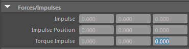
The following code is what we’ll use to control this attribute through the PyMel API:

body.attr('torqueImpulse').set(0.0, 0.0, float(action[0, 0]))

Creating the Rewards

Rewards measure the distance between the character’s current state and the desired goal. In the most basic examples of the DeepMimic paper the goal is to mimic a MoCap clip. Here we will use a joint as the goal. Using the equations in the paper as a reference I get:

(1) the angular distance between the RBD and the reference:

def getPoseRwd():
    ang_dist = body.attr('worldMatrix').get()._getRotate() * refBody.attr('worldMatrix').get()._getRotate().inverse()
    ang_dist = math.acos(min(1, ang_dist.w))
    return np.exp(-2*(ang_dis))

(2) the difference in angular velocity between RBD and reference:

def getVelocityRwd():
    body_prevWo = pmc.datatypes.Vector(body.getShapes()[1].attr('outPreSolverWorldRotate').get())
    body_currWo = pmc.datatypes.Vector(body.getShapes()[1].attr('outSolvedWorldRotate').get())
    velocity = body_currWo - body_prevWo
    velocity = np.sum(np.array(velocity))
    return np.exp(-.1*(velocity**2))

In the original paper the authors also reward the distance to the effectors and the COG, this is not applicable to this simplified example, but I have made the code for those available in the resources for this article. Finally, we combine these rewards using a weighted sum. The weights in the original paper are 0.65 for the pose reward, 0.1 for the velocity reward, 0.15 for the effector reward, and 0.1 for the COG reward. Here the weights are 0.6 for the pose reward and 0.4 for the velocity reward.

At this point, you can start testing the rewards in your simulated environment. Even if the reinforcement learning model is not yet implemented, you’ll see that calling getReward() should yield higher values for poses that are closer to the reference.

Creating the Neural Networks

As I have discussed in the video, this model entails the creation of two Neural Networks. The Policy Network is used to learn the best action for a given state. The Value Network is used to approximate the rewards provided by the actions taken previously. We then update the Policy Network in the direction that offers rewards that are superior to the values memorized by the Value Network.

I’ll be creating all the networks using Keras, inside Maya. We need to do this to use Maya’s Bullet plug-in to generate the data as we do the training. If you don’t know what Keras is or how to get it working inside Maya read this previous article first. For full disclosure, I’m using CNTK as Keras’ backend, as it has a GPU implementation that is easier to get working than Theano’s (IMHO).

I’ll also be using Keras’ Functional API, in opposition to the Sequential API that I have been using previously. The Sequential API is slightly more complicated but adds the flexibility that is needed for us to implement a custom loss function with rewards.

In the original paper, the Policy and Value nets have two hidden layers. In this straightforward example, one single layer is sufficient for everything that needs to be learned. The Value Neural Network is a very default net, please look-up the full code in the resources for its implementation. The Policy Network is slightly trickier. Here is the code for it:

def policy_model():
       # nn topology
       in_layer = layers.Input(shape=[n_inputs], name="input_x")
       h1_layer = layers.Dense(512,
                               activation="relu",
                               name="dense_1")(in_layer)
       out_layer = layers.Dense(n_outputs,
                                activation="linear",
                                name="out")(h1_layer)

       # advg_ph is a placeholder for inputing advantage value into
       # the model, making them available for the loss functions
       advg_ph = layers.Input(shape=[1], name="advantage")

       […]

First, we create the real layers: input, h1, and output. Note that how we connect one layer to another: new_layer = layers.type()(connected_layer).

Then we create a placeholder input layer for the advantage values (remember, advantage=reward-value). We leave this placeholder unconnected from the other layers. Finally, we build two networks, one for training (with the placeholder) and the other for prediction (without it):

       […]
       model_predict = Model(inputs=[in_layer], outputs=out_layer)
       model_train = Model(inputs=[in_layer, advg_ph], outputs=out_layer)
       […]

Since both networks link to the same layers in memory, any update we do in the training network happens in the prediction network as well. The only difference in both is that the training network receives an additional value (advantages). This trick is very Keras specific, and I must thank this guy for showing it.

For the loss function I got the Mean Squared Error function from Keras’ open source code and supplemented it with the advantages (stored in the advg_ph placeholder):

       […]
       def custom_loss(y_true, y_pred):
             return K.mean(advg_ph*K.square(y_pred - y_true), axis=-1)

Note that y_pred refers to the output of the network, while y_true is the output in the dataset.

So, what I’m doing here is multiplying the error by the advantage. If the advantage is high (near 1) it will minimize that error in; that is, we’ll move the policy towards this direction making such behavior more frequent in the future.

I then compile the training network using that custom loss function; please see the resources for the full code.

Creating the Training Loop

Reinforcement learning can’t be done all at once. We start from a random guess and try to steer learning towards states of higher returns. Hence, we simulate, train, rinse and repeat. Here is how this training loop looks overall:

for i in range(n_trains):
       # iniate variables in memory
       all_states = np.array([]).reshape(0, n_inputs).astype(np.float32)
       all_actions = np.array([]).reshape(0, n_outputs).astype(np.float32)
       all_rwds = all_dsc_rwds = np.array([]).reshape(0, 1).astype(np.float32)

       for j in range(n_episodes):
             # re/start simulation
             f = 0
             cmds.currentTime(f)
             ep_frames = ep_rwds = np.array([]).reshape(0, 1).astype(np.float32)

             while f < ep_size:
                    #things we do every frame

             # training the neural networks

Note that the simulation only stops when it reaches the end (f<ep_size). In the original paper, the episode may also end if the character reaches an early termination condition, like falling.

For every simulation frame we do the following things: (1) get the current state (the inputs for both networks), (2) predict an action from the policy network and jitter its results over a Gaussian distribution, (3) simulate the frame using that action, (4) evaluate the rewards, and (5) store results in memory.

                    # (1)
                    state = getState(root).astype(np.float32)

                    # (2)
                    action = policy_nn_predict.predict(state)
                    action = np.random.normal(action, deviation)  # jitter action

                    # (3)
                    root.attr('torqueImpulse').set(0.0, 0.0, float(action[0, 0]))
                    f += 1
                    cmds.currentTime(f)

                    # (4)
                    reward = np.float32(getReward())

                    # (5)
                    all_states = np.vstack([all_states, state])
                    all_actions = np.vstack([all_actions, action])
                    all_rwds = np.vstack([all_rwds, reward])
                    ep_rwds = np.vstack([ep_rwds, reward])

After we simulate one episode, we need to accumulate the discounted rewards. That is, for every frame, we sum the reward of all subsequent frames dampened by a particular discount. This spreads the contribution of an action over time since its effects may not be immediately apparent. The actual implementation of this is done in the discount_rewards() function, see full code in the resources.

After that we shuffle the samples, using the same seed for inputs, outputs, and rewards. This is necessary so that we can split validate our data into training and test sets, Keras won’t shuffle samples when doing this. Split validation is important to check if what is being learned about one part of the data set (the training set) generalizes well to the remainder of the samples (test set). If this is not the case, we can early stop that learning session to avoid overfitting. I have chosen to use split validation and early stopping to the training of the Value Network alone.

This is how you can shuffle samples:

       n_samples = all_states.shape[0]
       shuffle_ids = range(n_samples)
       np.random.shuffle(shuffle_ids)
       shuffle_states = np.ndarray(shape=(n_samples, all_states.shape[1]), dtype=np.float32)
[…]
       for idx, s_idx in zip(range(n_samples), shuffle_ids):
             shuffle_states[idx] = (all_states[s_idx])
[…]

This is how I train the Value Network with the randomized samples, validation splitting, and early stopping:

       early_stop_patient = keras.callbacks.EarlyStopping(patience=8)

       value_nn.fit(shuffle_states, shuffle_rwds,
                    verbose=2, validation_split=0.3, callbacks=[early_stop_patient],
                    epochs=n_epochs, batch_size=batch_size)

After training the Value Network, we can compare the actual rewards with approximated values to check if there are any advantageous samples for training the Policy Network:

       all_values = value_nn.predict(all_states)
       all_advg = np.maximum(0, all_dsc_rwds - all_values)
       all_advg /= np.max(all_advg)

Note that I keep the advantage values between zero and one because of the design of the loss function. Finally, we can train the Policy net:

       policy_nn_train.fit([all_states, all_advg], all_actions,
                              verbose=2, epochs=n_epochs, batch_size=batch_size)

For the full implementation check out the resources.

Training and evaluating the model

The training is slow compared to the models I have explained in previous tutorials, although applying it to this simple context is much faster than using it to learn the movements for a whole character. A big bottleneck in this implementation is querying and setting attributes in Maya through the Python API. If you set timers to evaluate the time elapsed in each process you will notice that the Neural Network predictions and the Bullet simulation are very cheap.

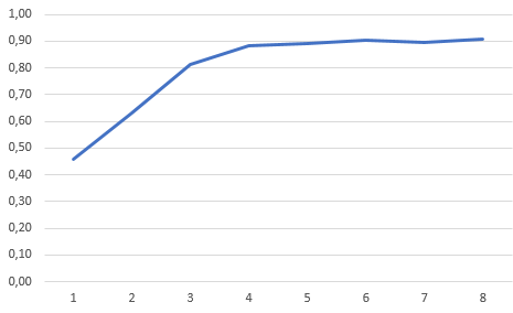
In the paper, the authors estimate that the average skill needs about 60,000,000 simulated frames to be learned, in about 14,500 training sessions. This is not something that would be practical with this Python prototype. For the example in the image below, I have trained the model over 8 sessions, generating 6,144 simulated frames. This took about 5 minutes.

In the plot below you can see that through the learning process the average performance goes up until it plateaus around the 6^th training session.

To evaluate the model, we can use our training loop removing the term that jitters the action.

f = 0
while f < 100:
       state = getState(root)

       action = policy_model_predict.predict(state)

       # eval sim
       root.attr('torqueImpulse').set(0.0, 0.0, float(action[0, 0]))

       f += 1
       cmds.currentTime(f)

If you want to save and load the model, you can use keras.model.save() and keras.model.load_model() to do so. You only need to save and load the policy_model_predict network, as the value network and the policy_model_train network are only relevant in the training process.

This prediction part of the model can be implemented inside a DG Node, which will make it easier to integrate it in Maya’s workflow. If you want to see an example of how this can be done check out this previous article.

Conclusion

Reinforcement models are useful in contexts where a goal can be clearly defined, but too much data needs to be generated to cope with the immense variations in the environment. This has applications in physically based character animation, robotics, and it is also the most successful model for AI that plays games (think of computers beating humans at Go or DOTA). This example was a gentle primer to this approach; complex problems display high variance during training and demand more sophisticated techniques to stabilize it.

You can experiment with this approach, applying to new scenarios. Maybe slightly more complex ragdolls, composed of 2 or 3 joints. Or maybe, change the hinge type constraint to a six-dof constraint to experiment with the added complexity.

Resources needed for this tutorial