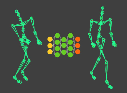
In this article, you’ll learn how to train an autoencoding Neural Network to compress and denoise motion capture data and display it inside Maya
Autoencoders are at the heart of some raytracer denoising and image upscaling (aka. super-resolution) technologies. Despite the pompous name, an autoencoder is just a Neural Network for which inputs and outputs are the same (except for the addition of noise, in some cases).
In this tutorial we’ll implement a simple autoencoder network and train it with MoCap data, then we’ll test it inside Autodesk Maya. Here are the things you’ll learn in this article:
- What is an autoencoder
- Loading kinematic (MoCap) data from a CSV to a Maya skeleton using a custom DG node
- Compressing data with an autoencoder
- Denoising data with an autoencoder
You’ll need these resources to follow this tutorial
What is an Autoencoder?
Autoencoder is a fancy name for a Neural Network that has a symmetric topology and for which inputs and outputs are the same. Why would anyone bother to train such a network, you might ask? Building such a network means you are creating an alternative way to represent the data in the hidden-neurons. This new representation may have useful characteristics: it may be more compact than the original representation (dimensionality reduction); it is data-driven and thus will encode common patterns from the data-set.
We can build autoencoders out of different topologies, such as fully-connected (which is the topology I have been using in most other tutorials), convolutional, recurrent, and so on. The input and output layers will have the same number of features, whatever that is; for the data going in and out should be the same. The hidden layers should, in theory, have fewer features than the input layer. This constraint exists because if the number of neurons in the hidden layers were equal to or greater than the inputs the network would learn to copy the inputs.
While this is ok if you want to build an auto-encoder for dimensionality reduction it is less than optimal if you’re going to use it for denoising since the dimensions in the hidden-layer will be capped. A way to get around this is to introduce sparsity into your training; I’ll talk more about this latter. First, we need some data to train this autoencoder.
Loading kinematic data (MoCap) from a CSV to a Maya skeleton using a custom DG node
For this tutorial, I have converted a subset of the CMU dataset into CSV files for your convenience (see the resources). The data consists mostly of locomotive movements from different subjects. Motions from subjects 38, 39, 40, and 41 are used for testing purposes only. Actions from subjects 07, 08, 09, 16, 35, and 69 are used for training and have been condensed into one Numpy variable for greater convenience. Both test and train data follow this pattern:
| Col 1 | Col 2 | Col 3 | Col 4 | Col 5 | Col 6 | Col 7 | Col 8 | Col 9 | Col 10 | Col 11 | Col 12… |
| Root position x | Root position y | Root position z | Root quaternion x | Root quaternion y | Root quaternion z | Root quaternion w | Bone 1 quaternion x | Bone 1 quaternion y | Bone 1 quaternion z | Bone 1 quaternion w | … |
This data structure is similar to what you would get from the original dataset in BVH format but using quaternions instead of Euler rotations. Training Neural Networks using Euler for rotations can be a bad idea since it is possible to express the same orientation with different combinations of angles.
To display this data in Maya we’ll use a skeleton that matches the one used in the CMU dataset (see resources), and a custom-built DG node that can read the CSV files and output them as 4×4 matrices that will, in turn, be used to control the skeleton. I’ve dealt with the basic building blocks for a custom Maya DG node in a previous post, so I highly encourage you to read that one first. I provide a template DG node in the resources so that you can follow along.
Creating the parameters
First, let’s create the Maya attributes needed for our node. All we need at first are a ‘file path’ to read from, a ‘frame’ so we can scrub through the animation, and a Matrix array to store the transforms for each of the joints of the character.
    # (1) Get Maya data types and attributes
    kString = om.MFnData.kString
    kFloat = om.MFnNumericData.kFloat
    tAttr = om.MFnTypedAttribute()
    nAttr = om.MFnNumericAttribute()
    mAttr = om.MFnMatrixAttribute()

    # (2) Setup attributes
    csvToMat.filePath = tAttr.create('filePath', 'fp', kString)
    tAttr.usedAsFilename = True
    csvToMat.frame = nAttr.create('frame','fr', kFloat, 0.0)
    nAttr.hidden = False
    nAttr.keyable = True
    csvToMat.matrixOut = mAttr.create('matOut', 'mo')
    mAttr.array = True
    mAttr.usesArrayDataBuilder = True

   # (3) Add the attributes to the node
    csvToMat.addAttribute(csvToMat.filePath)
    csvToMat.addAttribute(csvToMat.frame)
    csvToMat.addAttribute(csvToMat.matrixOut)

    # (4) Set the attribute dependencies
    csvToMat.attributeAffects(csvToMat.filePath, csvToMat.matrixOut)
    csvToMat.attributeAffects(csvToMat.frame, csvToMat.matrixOut)
Remember to add the attributes to the node (3) and to declare their dependencies (4).
Outside the functions that create and init the node, we will build a class to cache the CSV data once loaded. Then we create a global variable to start an object from this class and have it available for use inside the compute part of our node.
class DataCache:
    '''An interface for loading and caching data from CSV files'''
    filePath = ''
    data = None

    def getOrLoad(self, filePath):
        if filePath == self.filePath:
            return self.data
        self.filePath = filePath
        self.data = np.loadtxt(filePath, delimiter=',')

data_cache = DataCache()
Finally, we can declare our compute function, using attribute values to read from the data_cache object:
class csvToMat(om.MPxNode):
    '''A node for reading CSV files to Matrices.'''
    def compute(self, plug, data):
        # (1) Get handles from data stream
        fpHandle = data.inputValue(csvToMat.filePath)
        filePath = fpHandle.asString()
        frHandle = data.inputValue(csvToMat.frame)
        frame = int(np.float32(frHandle.asFloat()))
        matArrayHandle = data.outputArrayValue(csvToMat.matrixOut)
        matArrayBuilder = matArrayHandle.builder()

        # (2) Get CSV data and adjust number of matrices in array
        data_cache.getOrLoad(filePath)
        if type(data_cache.data) != type(None):
            n_xfos = (data_cache.data.shape[0]-3)/4
        else:
            n_xfos = 0
        n_ports = len(matArrayBuilder)
        if n_ports < n_xfos:
            for i in range(n_xfos-n_ports):
                matArrayBuilder.addLast()
        elif n_ports > n_xfos:
            for i in range(n_ports - 1, n_xfos - 1, -1):
                print('remove port ' + str(i))
                matArrayBuilder.removeElement(i)
        matArrayHandle.set(matArrayBuilder)

        # (3) Load data based on frame
        frame = max(0, frame)
        frame = min(frame, data_cache.data.shape[1]-1)
        frame_data = data_cache.data[:, frame]
        global_data = frame_data[:7]
        pose_data = frame_data[7:]

        # (4) Set global xfo
        global_tr = global_data[:3]
        global_ori = global_data[3:]
        global_mvec = om.MVector(global_tr)
        global_mquat = om.MQuaternion(global_ori)

        matHandle = matArrayHandle.outputValue()
        xfo = om.MTransformationMatrix()
        xfo.setRotation(global_mquat)
        xfo.setTranslation(global_mvec, 4) # 4 == global space
        matHandle.setMMatrix(xfo.asMatrix())
        matArrayHandle.next()

        # (5) Set local joint orientations
        for i in range(n_ports-1):
            matHandle = matArrayHandle.outputValue()

            j=i*4
            x = pose_data[j]
            y = pose_data[j+1]
            z = pose_data[j+2]
            w = pose_data[j+3]

            mquat = om.MQuaternion((x, y, z, w))
            xfo.setRotation(mquat)
            matHandle.setMMatrix(xfo.asMatrix())
            matArrayHandle.next()
Here is a quick overview of the code above. After loading values from attributes, we load the CSV, which is cached if the filename has not changed. The number of ports in the node will be adjusted to fit the data available in the CSV, following pattern outlined in the table previously shown. The seven first columns refer to the global xfo (translation + orientation of the root joints), all remaining columns refer to quaternion orientations of the remaining joints.
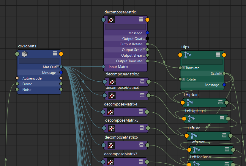
If the code is ok, you should be able to load one of the CSV files and connect it to the FBX skeleton. You’ll need to use ‘decompose matrix’ nodes to connect the output matrices to the proper transform components, like so:
If everything is setup correctly you should see something like this:
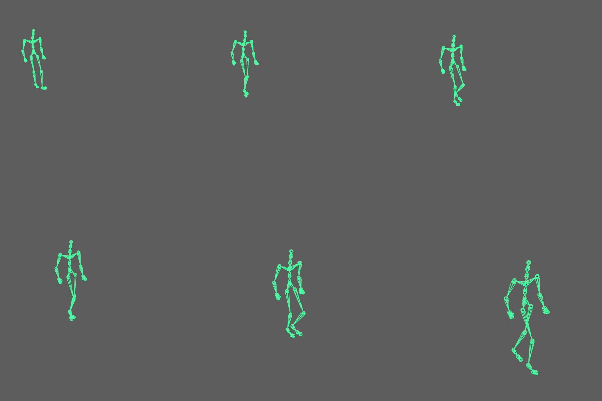
I provide you with a Maya scene in the resources, so you can see how everything should be connected.
Compressing data with an Autoencoder
Now that we can see the data, let us compress it using an Autoencoder. I provide you the Python code for that both in the form of regular .py files as well as Jupyter Notebooks (please check the resources for this article). Here I’ll go over the most cricital parts of the code.
data_folder = "../data/train"
data_file = os.path.join(data_folder,
                         'condensed_cmu_locomotion_dataset.npy')
data_container = np.load(data_file)
data_container = data_container[:,7:]
# Uncomment following lines to test and adjust hyperparameters
# np.random.shuffle(data_container)
# data_container = data_container[:1000,:]
The first thing we need to do, after loading the proper libraries, is to load the training dataset. Note that I am not using the first seven entries in the data container (root position and orientation) to train the network; the reason for that is to not teach the model to correlate global positioning with character poses, which would be wrong. Note that I have left commented out code you can use to train the network with a randomly chosen small sample of the data. It is good practice to check if your model works on little data, before having it working on big data, as training times differ a lot.
Now we set up the network’s topology:
input_dim = 120
encoding_dim1 = 60
encoding_dim2 = 30

input_data = Input(shape=(input dim,))
encode_h1 = Dense(encoding_dim1, activation='sigmoid')(input_data)
encode_h2 = Dense(encoding_dim2, activation='sigmoid')(encode_h1)
decode_h1 = Dense(encoding_dim1, activation='linear')(encode_h2)
decode_h2 = Dense(input_dim, activation='tanh')(decode_h1)
autoencoder = Model(input_data, decode_h2)
The input dimension is 120, one 4-dimensional quaternion for each of the 30 joints. Then we compress that to 60 features on the first hidden layer and down to 30 on the second one. The third hidden layer, or first decoding layer, brings the data back to 60 dimensions. And the final layer brings everything back to the original representation. A word about the activations: I’m using sigmoid activations to encode and linear activations to decode the data. This activation choice is a typical one in autoencoders, but it would work with other activations. The final activation “tanh” (aka tangential) is a bit of a trick related to the data we are using. The tanh layer fits activations to a range between -1 and 1, as has been discussed in this previous article. Quaternions also range from -1,1; so by using “tanh” we make sure we’ll get valid quaternion values without any post-processing step.
Now we compile and train the network.
adam = keras.optimizers.Adam(amsgrad=True)
autoencoder.compile(optimizer=adam, loss='mse')

train_history = autoencoder.fit(data_container, data_container,
                                epochs=2000,
                                batch_size=30000,
                                verbose=2)
Note that the inputs and outputs for our autoencoder are the same (data_container). This equality is a defining aspect of the autoencoder. To test our model in Maya, we save it:
autoencoder.save('autoenc_locomotion_pose_reduce.h5')
Loading the model in Maya
Then in Maya, we add some code to our custom node to load the model. We can do this very simply by loading the model to a global variable, in a hard-coded way:
autoencoder = load_model(os.path.join(
                         path, 'autoenc_locomotion_pose_reduce.h5'))
Then we can auto-encode the pose with our model by adding this line to the compute function:
encoded_data = autoencoder.predict(pose_data.reshape((1, 120)))
In the final code, available in the resources, you’ll note I have created a toggle parameter for autoencoding the data and a file path to load the model dynamically. It is a more elegant UI, but the idea is the same. Here is a comparison of the original data and the auto-encoded data:
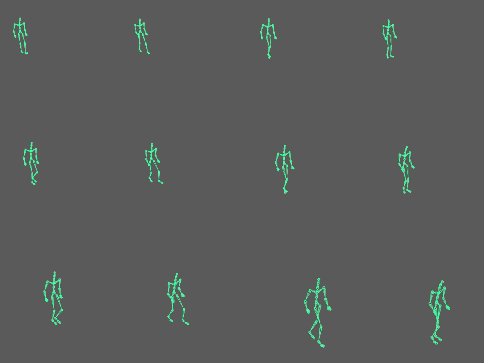
Note that it cannot match the input 100%, but keep in mind we are compressing the data by a factor of 4.
Denoising data with an autoencoder
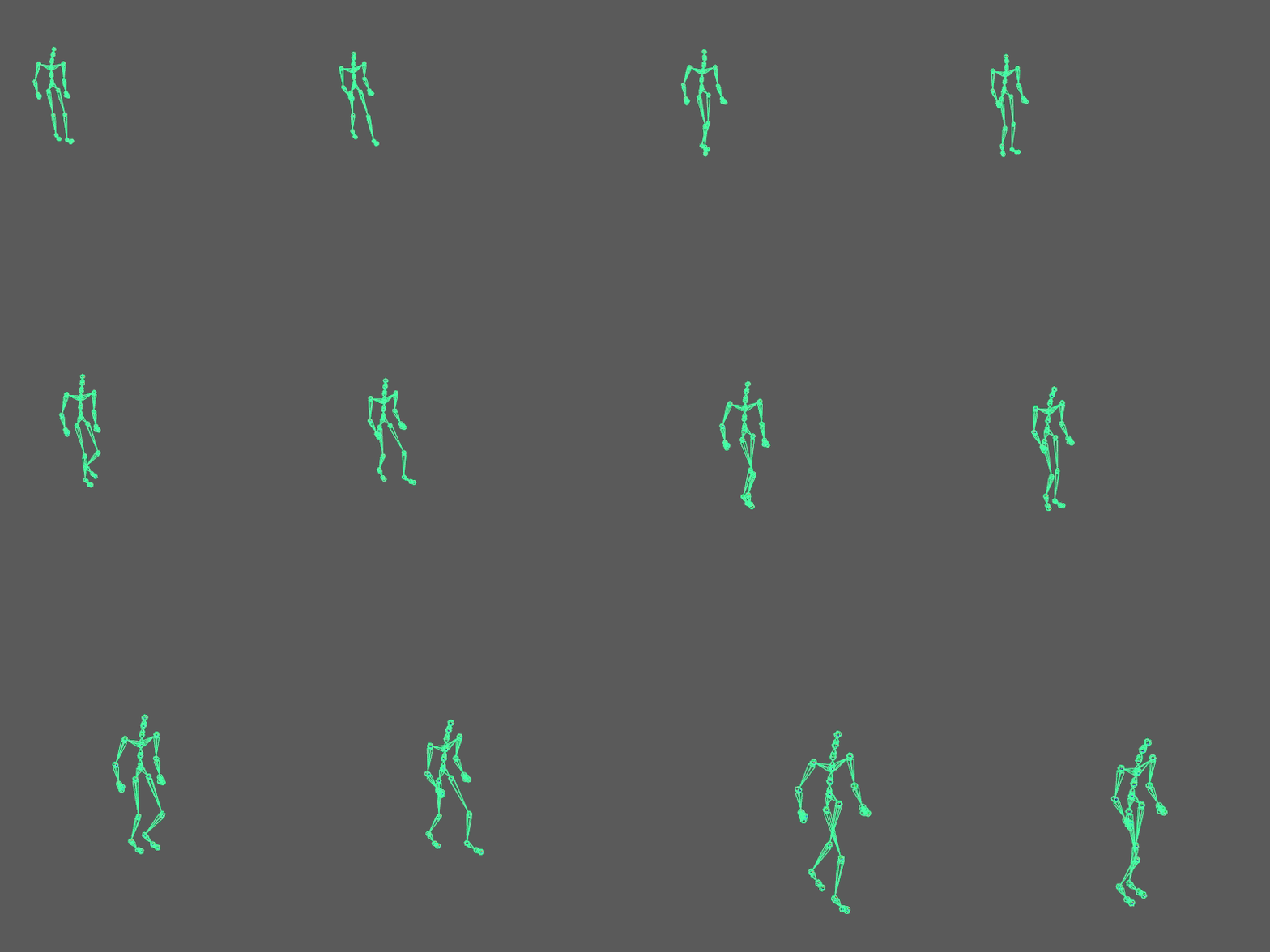
As the alternative representation of the pose emerges out of the recognition of patterns existent in the data, autoencoders tend to generate outputs that are built of components it has seen before. Hence, it enforces the reproduction of the structure of the original data and may remove unwanted artifacts such as noise (while introducing others such as blurring). We can put that to the test. For that we’ll create a noise parameter in our node:
    csvToMat.noise = nAttr.create('noise','no', kFloat, 0.0)
    nAttr.hidden = False
    nAttr.keyable = True
    nAttr.setSoftMin(0.0)
    nAttr.setSoftMax(0.01)
And then we use this noise value to add normally distributed noise to the pose:
        noHandle = data.inputValue(csvToMat.noise)
        noise_factor = np.float32(noHandle.asFloat())
  …
        np.random.seed(frame)
        noisy_pose = np.random.normal(pose_data, noise_factor)
Note that we seed the random samples with the frame number, so we can properly compare results. Finally, you’ll need to adjust the remainder of the compute function to use noisy_pose instead of pose_data, as can be seen in the final code available in the resources.
As you can see in the GIF below the autoencoder reduces the noise that we’ve artificially introduced.
Training autoencoders with sparsity
We may want to use an autoencoder exclusively for its denoising properties without any consideration for its dimensionality reduction capabilities. In that case, reducing dimensions can be a downside since we’ll limit the number of features our data representation is composed of and thus restrict its ability to learn how to represent the data. So, what we may want is to create an autoencoder that can have more dimensions in the hidden-layers than in the input and output layers. As I’ve explained before, this requires the introduction of some sparsity to the model. One way to add sparsity is to corrupt the inputs; another is to use penalties in the loss function. I’ll use the latter.
Here is how you add such a penalty in Keras:
input_dim = 120
encoding_dim1 = 256
encoding_dim2 = 128

l1 = keras.regularizers.l1(1e-9)

input_data = Input(shape=(120,))
encode_h1 = Dense(encoding_dim1, activation='sigmoid', activity_regularizer=l1)(input_data)
encode_h2 = Dense(encoding_dim2, activation='sigmoid')(encode_h1)
decode_h1 = Dense(encoding_dim1, activation='linear')(encode_h2)
decode_h2 = Dense(120, activation='tanh')(decode_h1)
autoencoder = Model(input_data, decode_h2)
L1 is a common sparsity-inducing penalty that is summed to the loss functions when you declare it in the activity_regularizer. In layman terms, what we do is induce fewer neurons to fire on any given stimulus, thus better isolating the learned features from one another. The amount of L1 added to the loss function (10e-9 in this case) directly impacts the training. Lower numbers will introduce less sparsity, the model will be more prone to overfitting, while larger numbers reduce the overfitting introducing more “blurriness” to the output of the network. Play with this value, give it a try.
Here is a comparison between the noisy data, the data auto-encoded with dimensionality reduction and the data auto-encoded with data expansion (and sparsity):

In Conclusion
In this article, you have learned what an autoencoder is and how to train one. Autoencoders have compression and denoising properties you can use in any data. Notice that our implementation is very simple and can only denoise a pose at a specific point in time, not accounting for previous and future poses. Expanding the model to account for such temporality would surely increase its precision and ability to denoise data.
You have also learned how to load kinematic data in Maya and pass it through a Neural Network using a custom DG node. This tooling is useful not only for autoencoders but for any other network you want to build to process MoCap data or Keyframe animations. You can also refactor this node to output data to CSV and build your own datasets.
