
Networks built out of one or many convolutional layers are the standard in image classification and are also used for other types of structured data. Understand how they work!
Convolutional neural network layers are readily available in frameworks such as Tensorflow, Theano, CNTK, and others. You don’t need to learn how to implement them yourself, but it is good practice to understand what they are doing. This article aims at providing an intuition for how these layers work in a (hopefully) sensible way and in under 800 words.
I assume you know what a neural network is, as CNNs are a particular case of that. If you don’t, please read this article first. With that out of the way let’s move on.
Why convolutions?
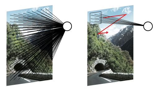
In a fully-connected topology, every dimension of the input affects every neuron in a given layer. This has an adverse effect in image classification (and other tasks): a feature learned in one part of an image (say the top right corner) won’t be classified when it appears in another region (anywhere but the top right corner). Features are learned with respect to their location in the input. In convolutional layers, the neurons are connected to a sliding window, which is translated and ‘fired’ over the whole input (see image below) making conv layers translation invariant.
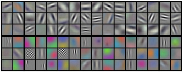
A convolutional layer may have one or many groups of neurons called kernels, or filters. Each filter is the size of the convolution’s sliding window. This is how filters look when a convolutional network is trained for image classification.
When a filter is applied to an image you get an output known as a feature map that looks something like this:
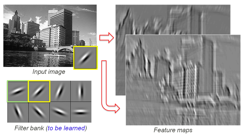
Each filter produces a corresponding feature map. In practice, each filter enhances some characteristic of the original image.
Now, how many neurons compose all these filters? And how big are those feature maps?
Let’s do some math. Say you have a 256×256 input with 3 color channels. You want to create a convolutional layer with a 3×3 sliding window and 8 filters. How many neurons are you training?
3 color channels * 3 pixels wide * 3 pixels tall * 8 filters = 216 neurons
Given those numbers, you will end up with 8 output feature maps. Their size is a bit trickier to calculate as it depends on the padding (how you treat image corners) and stride (how fast your window slides). The animation below can give you intuition on why bigger padding = bigger feature maps, and bigger stride = smaller feature maps. Check out the resources for more on this.
Ok, but what can we do with the resulting feature maps? One of three things:
- Convolute them again;
- Connect them to a fully connected layer;
- Down-res them before another convolution.
Pooling
In deep learning we want our networks to have two or more hidden-layers because we believe it can learn hierarchically; it should learn basic features first, and then other features built on top of those. The same applies to convolutional networks.
In images, features may be of different scales, some are tiny, others big. Therefore, it is useful to do convolutions at different resolutions. Going from small to large would be a good strategy as more prominent features will possibly be composed of smaller ones. There is where pooling comes in.
A pooling operation is just a down-res of the feature map outputted by a convolutional layer. This dimensionality reduction can be made by getting the average (average pooling) or maximum (max pooling) of the pixel values in a sliding window. When we convolute a pooled feature map, we can cover the features that exist in larger chunks of the image.
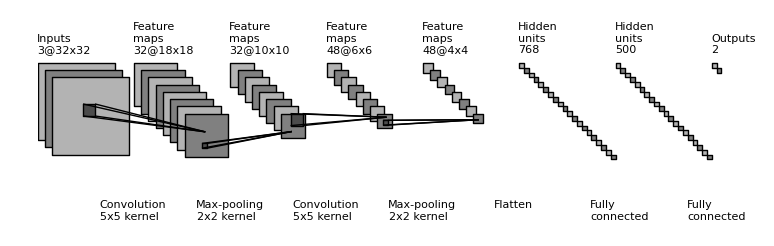
A typical topology for image classification is to combine Convolution + Pooling + Convolution + Pooling … until a fully connected layer is plugged at the end of the network.
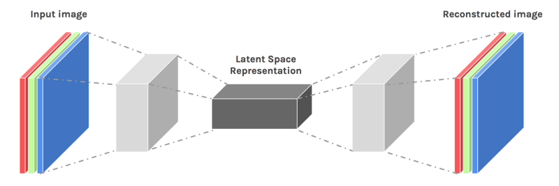
One can also deconvolute previously convoluted and pooled layers, by up-resing and convoluting the feature maps; effectively creating a convolutional autoencoder.
Applications
Convolutional networks were initially designed with the mammal visual cortex as an inspiration and are used all through image classification and generation tasks. But people have adapted its use to other types of structured data like 1d time-series and 3d voxels. In short convolution layers are useful anywhere you need translation invariance.
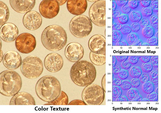
To exemplify convolutional networks in a CG context, I have created a tutorial on how to generate normal maps from color images, in a Substance like fashion. Check it out!
For more on the implementation and applications of convolutional networks check the resources for this article!